Produced by Charles Wells     Revised 2016-05-23

Introduction to this website    website TOC

website index   blog   head of Functions chapter
Functions can be represented visually in many different ways. There is a sharp difference between representing continuous functions and representing discrete functions.
For a continuous function $f$, $f(x)$ and $f(x')$ tend to be close together when $x$ and $x'$ are close together. That means you can represent the values at an infinite number of points by exhibiting a finite bunch of points that are so close together they appear to merge into a curve.
Nothing like this works for discrete functions. As you will see below, many different arrangements of the inputs and outputs can be made. In fact, different arrangements may be useful for representing different properties of the function.
The illustrations were created using these Mathematica Notebooks:
The most familiar representations of continuous functions are graphs of functions with one real variable. Students usually first see these in secondary school. Such representations are part of the subject called Analytic Geometry. This section gives examples of such functions.
The blue curve in the diagram below is a representation of the graph of the curve $g(x):=2-x^2$ for approximately the interval $(-2,2)$. The graph is the blue curve.
The brown right-angled line in the upper left side, for example, shows how the value of independent variable $x$ at $(0.5)$ is plotted on the horizontal axis, and the value of $g(0.5)$, which is $1.75$, is plotted on the vertical axis. So the blue graph contains the point $(0.5,g(0.5))=(0.5,1.75)$. The animated gif plotparmovie.gif shows a moving version of how the curve is plotted.
A discontinuous function which is continuous except for a small finite number of breaks can also be represented with a graph.
Below is a graph of (part of) the function $f:\mathbb{R}\to\mathbb{R}$ defined by\[f(x):=\left\{ \begin{align} 2-x^2\,\,\,\,\,\,\,\,\,\,\,\,\,\,\,\,\,\,\,\,\,\,(x\gt0) \\ 1-x^2\,\,\,\,\,\,(-1\lt x\lt 0) \\ 2-x^2\,\,\,\,\,\,\,\,\,\,\,\,\,\,\,\,\,(x\lt-1) \end{align}\right.\] $f$ is one function. It is defined for every real number except $-1$ and $0$.
Another discontinuous function is shown in Examples of functions
The Dirichlet function is defined by\[F(x):= \begin{cases} 1 & \text{if }x\text{ is rational}\\ \frac{1}{2} & \text{if }x\text{ is irrational}\\ \end{cases}\]for all real $x$.
It is impossible to draw a graph of this function, because it has an infinite number of gaps between its points. For more detail, see the article Examples of functions.
The graph of a continuous function cannot usually show the whole graph, unless it is defined only on a finite interval. This can lead you to jump to conclusions.
For example, you can't tell from the the graph of the function $y=2-x^2$ whether it has a local minimum (because the graph does not show all of the function), although you can tell by using calculus on the formula that it does not have one. The graph looks like it might have a vertical asymptotes, but it doesn't, again as you can tell from the formula (it is defined for all real numbers).
Discovering facts about a function
by looking at its graph
is useful but dangerous.
Below is the graph of the function\[f(x)=.0002{{\left( \frac{{{x}^{3}}-10}{3{{e}^{-x}}+1} \right)}^{6}}\]
If you didn't know the formula for the function, by looking at the graph you might nevertheless suspect certain things are true of the function.
If you do know the formula, you can find out many things about the function that you can't depend on the graph to see.
The section on Zooming and Chunking gives other details.
Suppose $F:\mathbb{R}\to\mathbb{R}\times\mathbb{R}$. That means you put in one number and get out a pair of numbers.
An example is the unit circle, which is the graph of the continuous function $t\mapsto(\cos t,\sin t)$. That has this parametric plot:
Because $\cos^2 t+\sin^2 t=1$, every real number $t$ produces a point on the unit circle. Four point are shown. For example,\[(\cos\pi,\,\sin\pi)=(-1,0)\] and \[(\cos(5\pi/3),\,\sin(5\pi/3))=(\frac{1}{2},\frac{\sqrt3}{2})\approx(.5,.866)\]
In graphing functions $f:\mathbb{R}\to\mathbb{R}$, the plot is in two dimensions and consists of the points $(x,f(x))$: the input and the output. The parametric plot shown above for $t\mapsto(\cos^2 t+\sin^2)$ shows only the output points $(\cos t,\sin t)$; $t$ is not plotted on the graph at all. So the graph is in the plane instead of in three-dimensional space.
It is useful to think of $t$ as time. If you start at some number $t$ on the real line and continually increase it, the value $f(t)$ moves around the circle counterclockwise, repeating every $2\pi$ times. If you decrease $t$, the value moves clockwise. The animated gif circlemovie.gif shows how the location of a point on the circle moves around the circle as $t$ changes from $0$ to $2\pi$. Every point is traversed an infinite number of times as $t$ runs through all the real numbers.
This is the parametric graph of the function $t\mapsto(\cos t,\sin 2t)$.
Notice that it crosses itself at the origin when $t$ is any odd multiple of $\frac{\pi}{2}$.
The graph of a function from a subset of $\mathbb{R}$ to $\mathbb{R}\times\mathbb{R}\times\mathbb{R}$ can also be drawn as a parametric graph in three-dimensional space, giving a three-dimensional curve.
Here is a view of the graph of the function \[t\mapsto(\cos t, \sin t, \sin 7t):\mathbb{R}\to \mathbb{R}\times\mathbb{R}\times\mathbb{R}\]
The animated gif crownmovie.gif represents the parameter $t$ in time.
Since we have access to three dimensions, we can display on the graph the input $t$ to the unit circle function $(\cos t,\sin t)$ by using a three-dimensional graph, shown below. The blue circle is the function $t\mapsto(\cos t,\sin t,0)$ and the gold helix is the function $t\mapsto(\cos t,\sin t,.2t)$.
The introduction of $t$ as the value in the vertical direction changes the circle into a helix. The animated .gif covermovie.gif shows both the travel of a point on the circle and the corresponding point on the helix.
As $t$ changes, the circle is drawn over and over with a period of $2\pi$. Every point on the circle is traversed an infinite number of times as $t$ runs through all the real numbers. But each point on the helix is traversed exactly once. For a given value of $t$, the point on the helix is always directly above or below the point on the circle.
The helix is called the universal covering space of the circle, and the set of points on the helix over (and under) a particular point $p$ on the circle is called the fiber over $p$. The universal cover of a space is a big deal in topology.
Here are two views of the function \[t\mapsto(\cos t,\sin 2t, \log t):\mathbb{R^{+}}\to \mathbb{R}\times\mathbb{R}\times\mathbb{R}\] ($\mathbb{R}^{+}$ is the set of positive real numbers)
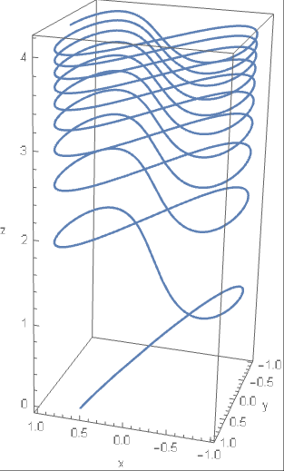
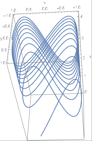
It is a universal cover (with an added squish as $z$ increases) of the Figure-8 curve.
The graph of a map $\mathbb{R}^m\to\mathbb{R}^n$ where $m+n\gt3$ requires $m+n$ dimensions, so we can't draw it and it is difficult to visualize it.
You can graph a function $\mathbb{R}\times\mathbb{R}\to\mathbb{R}\times\mathbb{R}$ using its endograph.
The function \[(x,y)\mapsto(x+.5,y+.2)\] moves each point in the plane $.5$ units to the right and $.2$ units up. The endograph below visualizes a part of this action. showing the movement at each point with integer coordinates.
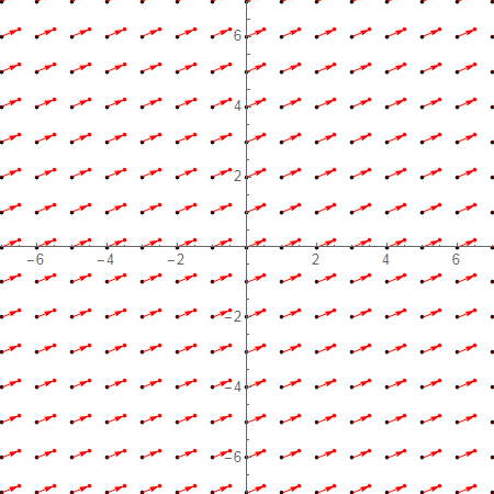
This is an example of an affine map in the plane.
The linear map determined by the matrix \[\pmatrix{1.25 & 0.5\\0.5&1}\] defines a function \[(x,y)\mapsto (1.25x+.5y,\,.5x+y):\mathbb{R}\times \mathbb{R}\to \mathbb{R}\times \mathbb{R}\] that can be displayed with an endograph like this:
Complex functions are often graphed using $\mathbb{R}\times\mathbb{R}$ for the domain (representing $a+bi$ as $(a,b)$), with the values of the function shown as hue and brightness, as seen in the Wikipedia article.
Complex analysis, the theory of functions on the complex numbers, is one of the richest and most highly developed parts of math.
This is the graph of part of the surface\[(x,y)\mapsto(x,z,\sin xz):\mathbb{R}\times\mathbb{R}\to\mathbb{R}\times\mathbb{R}\times\mathbb{R}\]

The blue curves follow the shape of the surface as an aid to visualizing the surface.
This graph was created by the Mathematica notebook AnotherFamiliesFrozen.nb It is worthwhile viewing this notebook in CDF Player, if you have it. (It is free). There are more examples in Freezing a family of functions.
When a function is continuous, its graph shows up as a curve in the plane or as a curve or surface in 3D space. When a function is defined on a set without any notion of continuity (for example a finite set), the graph is just a set of ordered pairs and does not tell you much.
A finite function $f:S\to T$ may be represented in these ways:
All these techniques can also be used to show finite portions of infinite discrete functions, but that possibility will not be discussed here.
Let \[\text{f}:\{a,b,c,d,e\}\to\{a,b,c,d\}\] be the function defined by requiring that $\text{f}(a)=c$, $\text{f}(b)=a$, $\text{f}(c)=c$, $\text{f}(d)=b$, and $\text{f}(e)=d$.
The graph of $\text{f}$ is the set \[(a,c),(b,a),(c,c),(d,b),(e,d)\] As with any set, the order in which the pairs are listed is irrelevant. Also, the letters $a$, $b$, $c$, $d$ and $e$ are merely letters. They are not variables.
$\text{f}$ is given by this table:

This sort of table is the format used in databases. For example, a table in a database might show the department each employee of a company works in:

The rule determined by the finite function $\text{f}$ has the form
\[(a\mapsto b,b\mapsto a,c\mapsto c,d\mapsto b,e\mapsto d)\]Rules are built in to Mathematica and are useful in many situations. In particular, the endographs in this article are created using rules. In Mathematica, however, rules are written like this:
\[(a\to b,b\to a,c\to c,d\to b,e\to d)\]This is inconsistent with the usual math usage (see barred arrow notation) but on the other hand is easier to enter when using Mathematica.
In fact, Mathematica uses very short arrows in their notation for rules, shorter than the ones used for the arrow notation for functions. Those extra short arrows don't seems to exist in TeX.
Two-line notation is a kind of horizontal table.
\[\begin{pmatrix} a&b&c&d&e\\c&a&c&b&d\end{pmatrix}\]The three notations table, rule and two-line do the same thing: If $n$ is in the domain, $\text{f}(n)$ is shown adjacent to $n$ -- to its right for the table and the rule, and below it for the two-line.
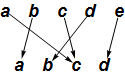
To make the cograph of a finite function, you list the domain and codomain in separate parallel rows or columns (even if the domain and codomain are the same set), and draw an arrow from each $n$ in the domain to $\text{f}(n)$ in the codomain.
This is the cograph for $\text{f}$, represented in columns
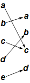
and in rows
Pretty ugly, but the cograph for finite functions does have its uses, as for example in the Wikipedia article composition of functions.
In contrast to the table, rule and two-line notation, in a cograph each element of the codomain is shown only once, even if the function is not injective.
In both the two-line notation and in cographs displayed vertically, the function goes down from the domain to the codomain. I guess functions obey the law of gravity.
There is no expectation that in the cograph $f(n)$ will be adjacent to $n$. But in most cases you can rearrange both the domain and the codomain so that some of the structure of the function is made clearer; for the function $\text{f}$:
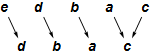
The domain and codomain of a finite function can be rearranged in any way you want because finite functions are not continuous functions. This means that the locations of points $x_1$ and $x_2$ have nothing to do with the locations of $f(x_1)$ and $f(x_2)$: The domain and codomain are discrete.
The endograph of a function $h:S\to T$ contains one node labeled $s$ for each $s\in S\cup T$, and an arrow from $s$ to $s'$ if $h(s)=s'$. Below is the endograph for $\text{f}$.

The endograph shows you immediately that $\text{f}$ is not a permutation. You can also see that with whatever letter you start with, you will end up at $c$ and continue looping at $c$ forever. You could have figured this out from the cograph (especially the rearranged cograph above), but it is not immediately obvious in the cograph the way it in the endograph.
There are more examples of endographs below and in the blog post A tiny step towards killing string-based math. Calculus-type functions can also be shown using endographs and cographs: See Mapping Diagrams from A(lgebra) B(asics) to C(alculus) and D(ifferential) E(quation)s, by Martin Flashman, and my blog posts Endographs and cographs of real functions and Demos for graph and cograph of calculus functions.
Suppose $p$ is the permutation of the set \[\{0,1,2,3,4,5,6,7,8,9\}\]given in two-line form by \[\begin{pmatrix} 0&1&2&3&4&5&6&7&8&9\\0&2&1&4&5&3&7&8&9&6\end{pmatrix}\]
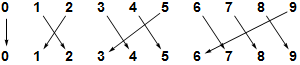
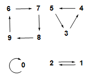
Again, the endograph shows the structure of the function much more clearly than the cograph does.
The endograph consists of four separate parts (called components) not connected with each other. Each part shows that repeated application of the function runs around a kind of loop; such a thing is called a cycle. Every permutation of a finite set consists of disjoint cycles as in this example.
Any permutation of a finite set can be represented in disjoint cycle notation: The function $p$ is represented by:
\[(0)(1,2)(3,4,5)(6,7,8,9)\]Given the disjoint cycle notation, the function can be determined as follows: For a given entry $n$, $p(n)$ is the next entry in the notation, if there is a next entry (instead of a parenthesis). If there is not a next entry, $p(n)$ is the first entry in the cycle that $n$ is in. For example, $p(7)=8$ because $8$ is the next entry after $7$, but $p(5)=3$ because the next symbol after $5$ is a parenthesis and $3$ is the first entry in the same cycle.
The disjoint cycle notation is not unique for a given permutation. All the following notations determine the same function $p$:
\[(0)(1,2)(4,5,3)(6,7,8,9)\] \[(0)(1,2)(8,9,6,7)(3,4,5)\] \[(1,2)(3,4,5)(0)(6,7,8,9)\] \[(2,1)(5,3,4)(9,6,7,8)\] \[(5,3,4)(1,2)(6,7,8,9)\]Cycles such as $(0)$ that contain only one element are usually omitted in this notation.
The article Images and Metaphors for Functions contains a detailed example of representations of a permutation.
Below is the endograph of a function \[t:\{0,1,2,3,4,5,6,7,8,9\}\to\{0,1,2,3,4,5,6,7,8,9\}\]
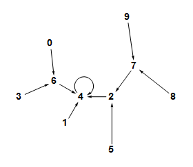
This endograph is a tree. The graph of a function $f$ is a tree if the domain has a particular element $r$ called the root with the properties that
In the case of $t$, the root is $4$. Note that $t(4)=4$, $t(t(7))=4$, $t(t(t(9)))=4$, $t(1)=4$, and so on.
You may complain that I didn't define the function that made the tree above. Well, I don't have to. The tree itself defines the function. All the ways of exhibiting finite functions that I have discussed here tell you exactly what the function is (except in some cases what the codomain is).
The endograph
shown above is also a tree.
See the Wikipedia article on trees for the usual definition of tree as a special kind of graph. For reading this article, the definition given in the previous paragraph is sufficient.
This is the endograph of a function $t$ on a $17$-element set:
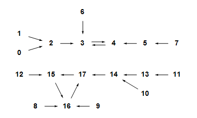
It has two components. The upper one contains one $2$-cycle, and when you apply $t$ over and over to any point in that component, you wind up flipping back and forth in the $2$-cycle forever. The lower component has a $3$-cycle with a similar property.
This illustrates a general fact about finite functions:
In the example above, the cycle in the top component has three trees attached to it, two to $3$ and one to $4$, and the cycle in the bottom component has four trees attached to it.
You can check your understanding of finite functions by thinking about the following two theorems:
This work is licensed under a Creative Commons Attribution-ShareAlike 2.5 License.