Introduction to this post
I am writing a new abstractmath chapter called Representations of Functions. It will replace some of the material in the chapter Functions: Images, Metaphors and Representations. This post is a draft of the sections on representations of finite functions.
The diagrams in this post were created using the Mathematica Notebook Constructions for cographs and endographs of finite functions.nb.
You can access this notebook if you have Mathematica, which can be bought, but is available for free for faculty and students at many universities, or with Mathematica CDF Player, which is free for anyone and runs on Windows, Mac and Linux.
Like everything in abstractmath.org, the notebooks are covered by a Creative Commons ShareAlike 3.0 License.
Segments posted so far
Graphs of finite functions
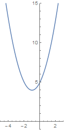
When a function is continuous, its graph shows up as a curve in the plane or as a curve or surface in 3D space. When a function is defined on a set without any notion of continuity (for example a finite set), the graph is just a set of ordered pairs and does not tell you much.
A finite function $f:S\to T$ may be represented in these ways:
- Its graph $\{(s,f(s))|s\in S\}$. This is graph as a mathematical object, not as a drawing or as a directed graph — see graph (two meanings)).
- A table, rule or two-line notation. (All three of these are based on the same idea, but differ in presentation and are used in different mathematical specialties.)
- By using labels with arrows between them, arranged in one of two ways:
- A cograph, in which the domain and the codomain are listed separately.
- An endograph, in which the elements of the domain and the codomain are all listed together without repetition.
All these techniques can also be used to show finite portions of infinite discrete functions, but that possibility will not be discussed here.
Introductory Example
Let \[\text{f}:\{a,b,c,d,e\}\to\{a,b,c,d\}\] be the function defined by requiring that $f(a)=c$, $f(b)=a$, $f(c)=c$, $f(d)=b$, and $f(e)=d$.
Graph
The graph of $f$ is the set
\[(a,c),(b,a),(c,c),(d,b),(e,d)\]
As with any set, the order in which the pairs are listed is irrelevant. Also, the letters $a$, $b$, $c$, $d$ and $e$ are merely letters. They are not variables.
Table
$\text{f}$ is given by this table:

This sort of table is the format used in databases. For example, a table in a database might show the department each employee of a company works in:

Rule
The rule determined by the finite function $f$ has the form
\[(a\mapsto b,b\mapsto a,c\mapsto c,d\mapsto b,e\mapsto d)\]
Rules are built in to Mathematica and are useful in many situations. In particular, the endographs in this article are created using rules. In Mathematica, however, rules are written like this:
\[(a\to b,b\to a,c\to c,d\to b,e\to d)\]
This is inconsistent with the usual math usage (see barred arrow notation) but on the other hand is easier to enter in Mathematica.
In fact, Mathematica uses very short arrows in their notation for rules, shorter than the ones used for the arrow notation for functions. Those extra short arrows don’t seems to exist in TeX.
Two-line notation
Two-line notation is a kind of horizontal table.
\[\begin{pmatrix} a&b&c&d&e\\c&a&c&b&d\end{pmatrix}\]
The three notations table, rule and two-line do the same thing: If $n$ is in the domain, $f(n)$ is shown adjacent to $n$ — to its right for the table and the rule and below it for the two-line.
Note that in contrast to the table, rule and two-line notation, in a cograph each element of the codomain is shown only once, even if the function is not injective.
Cograph
To make the cograph of a finite function, you list the domain and codomain in separate parallel rows or columns (even if the domain and codomain are the same set), and draw an arrow from each $n$ in the domain to $f(n)$ in the codomain.
This is the cograph for $\text{f}$, represented in columns
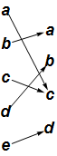
and in rows (note that $c$ occurs only once in the codomain)
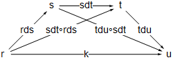
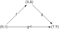
Pretty ugly, but the cograph for finite functions does have its uses, as for example in the Wikipedia article composition of functions.
In both the two-line notation and in cographs displayed vertically, the function goes down from the domain to the codomain. I guess functions obey the law of gravity.
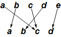
Rearrange the cograph
There is no expectation that in the cograph $f(n)$ will be adjacent to $n$. But in most cases you can rearrange both the domain and the codomain so that some of the structure of the function is made clearer; for example:
The domain and codomain of a finite function can be rearranged in any way you want because finite functions are not continuous functions. This means that the locations of points $x_1$ and $x_2$ have nothing to do with the locations of $f(x_1)$ and $f(x_2)$: The domain and codomain are discrete.
Endograph
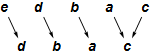
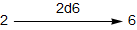
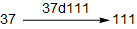
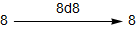
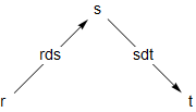
The endograph of a function $f:S\to T$ contains one node labeled $s$ for each $s\in S\cup T$, and an arrow from $s$ to $s’$ if $f(s)=s’$. Below is the endograph for $\text{f}$.

The endograph shows you immediately that $\text{f}$ is not a permutation. You can also see that with whatever letter you start with, you will end up at $c$ and continue looping at $c$ forever. You could have figured this out from the cograph (especially the rearranged cograph above), but it is not immediately obvious in the cograph the way it in the endograph.
There are more examples of endographs below and in the blog post
A tiny step towards killing string-based math. Calculus-type functions can also be shown using endographs and cographs: See Mapping Diagrams from A(lgebra) B(asics) to C(alculus) and D(ifferential) E(quation)s, by Martin Flashman, and my blog posts Endographs and cographs of real functions and Demos for graph and cograph of calculus functions.
Example: A permutation
Suppose $p$ is the permutation of the set \[\{0,1,2,3,4,5,6,7,8,9\}\]given in two-line form by
\[\begin{pmatrix} 0&1&2&3&4&5&6&7&8&9\\0&2&1&4&5&3&7&8&9&6\end{pmatrix}\]
Cograph
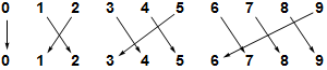
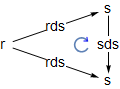
Endograph
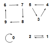
Again, the endograph shows the structure of the function much more clearly than the cograph does.
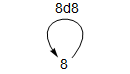
The endograph consists of four separate parts (called components) not connected with each other. Each part shows that repeated application of the function runs around a kind of loop; such a thing is called a cycle. Every permutation of a finite set consists of disjoint cycles as in this example.
Disjoint cycle notation
Any permutation of a finite set can be represented in disjoint cycle notation: The function $p$ is represented by:
\[(0)(1,2)(3,4,5)(6,7,8,9)\]
Given the disjoint cycle notation, the function can be determined as follows: For a given entry $n$, $p(n)$ is the next entry in the notation, if there is a next entry (instead of a parenthesis). If there is not a next entry, $p(n)$ is the first entry in the cycle that $n$ is in. For example, $p(7)=8$ because $8$ is the next entry after $7$, but $p(5)=3$ because the next symbol after $5$ is a parenthesis and $3$ is the first entry in the same cycle.
The disjoint cycle notation is not unique for a given permutation. All the following notations determine the same function $p$:
\[(0)(1,2)(4,5,3)(6,7,8,9)\]
\[(0)(1,2)(8,9,6,7)(3,4,5)\]
\[(1,2)(3,4,5)(0)(6,7,8,9)\]
\[(2,1)(5,3,4)(9,6,7,8)\]
\[(5,3,4)(1,2)(6,7,8,9)\]
Cycles such as $(0)$ that contain only one element are usually omitted in this notation.
Example: A tree
Below is the endograph of a function \[t:\{0,1,2,3,4,5,6,7,8,9\}\to\{0,1,2,3,4,5,6,7,8,9\}\]
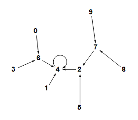
This endograph is a tree. The graph of a function $f$ is a tree if the domain has a particular element $r$ called the root with the properties that
- $f(r)=r$, and
- starting at any element of the domain, repreatedly applying $f$ eventually produces $r$.
In the case of $t$, the root is $4$. Note that $t(4)=4$, $t(t(7))=4$, $t(t(t(9)))=4$, $t(1)=4$, and so on.
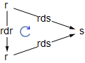
The endograph
shown here is also a tree.
See the Wikipedia article on trees for the usual definition of tree as a special kind of graph. For reading this article, the definition given in the previous paragraph is sufficient.
The general form of a finite function
This is the endograph of a function $t$ on a $17$-element set:
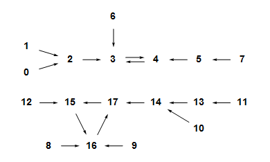
It has two components. The upper one contains one $2$-cycle, and no matter where you start in that component, when you apply $t$ over and over you wind up flipping back and forth in the $2$-cycle forever. The lower component has a $3$-cycle with a similar property.
This illustrates a general fact about finite functions:
- The endograph of any finite function contains one or more components $C_1$ through $C_k$.
- Each component $C_k$ contains exactly one $n_k$ cycle, for some integer $n_k\geq 1$, to which are attached zero or more trees.
- Each tree in $C_k$ is attached in such a way that its root is on the unique cycle contained in $C_k$.
In the example above, the top component has three trees attached to it, two to $3$ and one to $4$. (This tree does not illustrate the fact that an element of one of the cycles does not have to have any trees attached to it).
You can check your understanding of finite functions by thinking about the following two theorems:
- A permutation is a finite function with the property that its cycles have no trees attached to them.
- A tree is a finite function that has exactly one component whose cycle is a $1$-cycle.

This work is licensed under a Creative Commons Attribution-ShareAlike 2.5 License.
 Send to Kindle
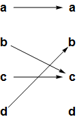


